An Introduction to XGBoost R package
Introduction
XGBoost is a library designed and optimized for boosting trees algorithms. Gradient boosting trees model is originally proposed by Friedman et al. The underlying algorithm of XGBoost is similar, specifically it is an extension of the classic gbm algorithm. By employing multi-threads and imposing regularization, XGBoost is able to utilize more computational power and get more accurate prediction. Please refer to this tutorial for the details of the model.
One evidence of its accuracy is that XGBoost is used in more than half of the winning solutions in machine learning challenges hosted at Kaggle. We have prepared a (incomplete) list of winning solutions.
There’re various high-level interfaces. Currently there are interfaces of XGBoost in C++, R, python, Julia, Java and Scala. The core functions in XGBoost are implemented in C++, thus it is easy to share models among different interfaces. This post is going to focus on the R package xgboost, which has a friendly user interface and comprehensive documentation. Based on the statistics from the RStudio CRAN mirror, The package has been downloaded for more than 4,000 times in the last month.
The R package xgboost has won the 2016 John M. Chambers Statistical Software Award. From the very beginning of the work, our goal is to make a package which brings convenience and joy to the users. Thus we will introduce several details of the R pacakge xgboost that (we think) users would love to know.
A 1-minute Beginner’s Guide
xgboost is available on both CRAN and Github. To install the stable/pre-compiled version from CRAN, simply run:
install.packages('xgboost')
You can also install from our weekly updated drat repo:
install.packages("drat", repos="https://cran.rstudio.com")
drat:::addRepo("dmlc")
install.packages("xgboost", repos="http://dmlc.ml/drat/", type="source")
In order to run a machine learning algorithm, we need a data set first. xgboost has a demo data set about mushrooms. This data set records biological attributes of different mushroom species, and the target is to predict whether it is poisonous. Users can load the data with
require(xgboost)

data(agaricus.train, package='xgboost')
data(agaricus.test, package='xgboost')
train <- agaricus.train
test <- agaricus.test
Each variable is a list containing two things, label and data. The next step is to feed this data to xgboost. Besides the data, we need to train the model with some other parameters:
nrounds: the number of decision trees in the final modelobjective: the training objective to use, where “binary:logistic” means a binary classifier.
The simplest training command is as follows:
model <- xgboost(data = train$data, label = train$label,
                 nrounds = 2, objective = "binary:logistic")
## [0]	train-error:0.000614
## [1]	train-error:0.001228
We can make prediction on the test data set easily:
preds = predict(model, test$data)
Sometimes it is important to use cross-validation to exam our model. In xgboost we provide a function xgb.cv to do that. Basically users can just copy every thing from xgboost, and specify nfold:
cv.res <- xgb.cv(data = train$data, label = train$label, nfold = 5,
                 nrounds = 2, objective = "binary:logistic")
## [0]	train-error:0.000921+0.000343	test-error:0.001228+0.000687
## [1]	train-error:0.001075+0.000172	test-error:0.001228+0.000687
To get to know more details about the usage of xgboost, please visit our tutorial for more information.
Efficient Algorithm
If you have experiences in training models on a large data set, then you probably agree that waiting for the training to be done is boring. Time is a resource, so the training speed of an learning algorithm is important. This is determined by both algorithm and implementation. We pay attention to these issues when building xgboost, thus we are confident that xgboost is one of the fastest learning algorithm of gradient boosting algorithm. The reasons for the good efficiency are:
- The computational part is implemented in C++.
- It can be multi-threaded on a single machine.
- It preprocesses the data before the training algorithm.
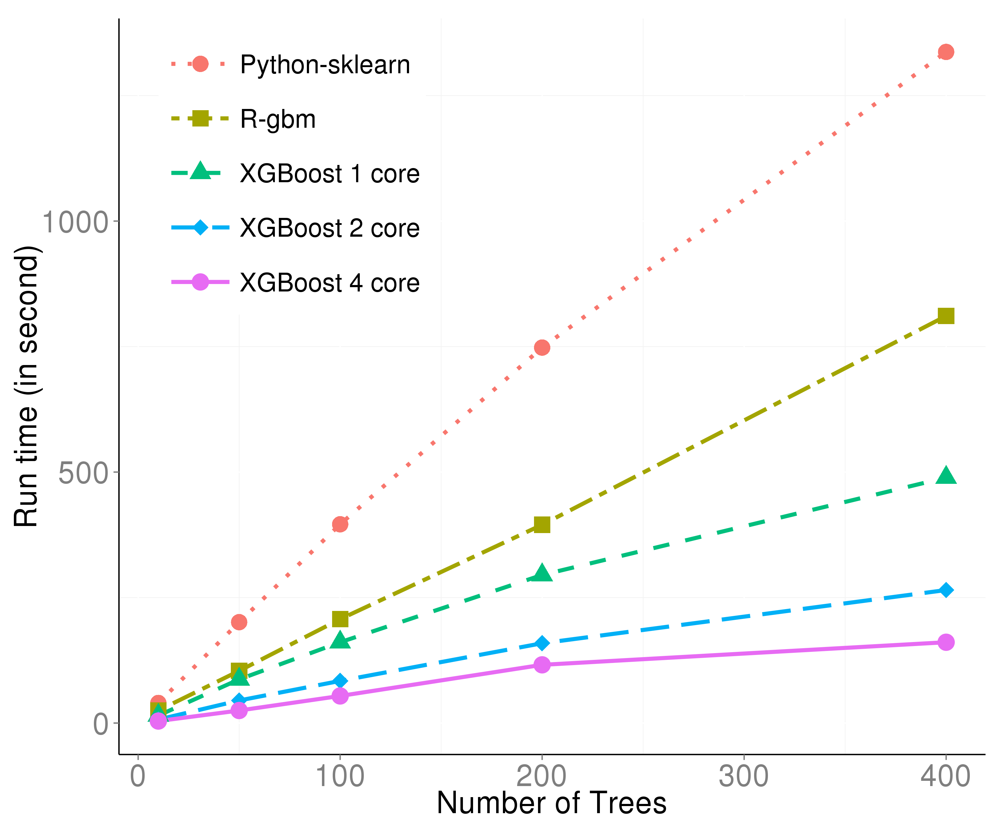
This figure is generated with the dataset from the Higgs Boson Competition. It can be described from two aspects:
- With only one thread, the effect of preprocessing and C++ is already obvious.
- The multi-threading is almost linear with the number of threads, thus boosting the efficiency further.
Convenient Interface
As the developers of xgboost, we are also heavy users of xgboost. We value the experience on this tool. During the development, we try to shape the package to be user-friendly. Here are several details we would like to share, please click the title to visit the sample code.
Customized Objective
xgboost can take customized objective. This means the model could be trained to optimize the objective defined by user. This is not often seen in other tools, since most of the algorithms are binded with a specific objective. With xgboost, one can train a model which maximize the work on the correct direction.
Let’s use log-likelihood as an demo. We define the following function to calculate the first and second order of gradient of the loss function:
loglossobj <- function(preds, dtrain) {
  # dtrain is the internal format of the training data
  # We extract the labels from the training data
  labels <- getinfo(dtrain, "label")
  # We compute the 1st and 2nd gradient, as grad and hess
  preds <- 1/(1 + exp(-preds))
  grad <- preds - labels
  hess <- preds * (1 - preds)
  # Return the result as a list
  return(list(grad = grad, hess = hess))
}
Then we train the model as
model <- xgboost(data = train$data, label = train$label,
                 nrounds = 2, objective = loglossobj, eval_metric = "error")
## [0]	train-error:0.001228
## [1]	train-error:0.001228
The result should be equivalent to objective = "binary:logistic".
Early Stopping
A usual scenario is when we are not sure how many trees we need, we will firstly try some numbers and check the result. If the number we try is too small, we need to make it larger; If the number is too large, we are wasting time to wait for the termination. By setting the parameter early_stopping, xgboost will terminate the training process if the performance is getting worse in the iteration.
bst <- xgb.cv(data = train$data, label = train$label, nfold = 5,
              nrounds = 20, objective = "binary:logistic",
              early.stop.round = 3, maximize = FALSE)
## [0]	train-error:0.000921+0.000343	test-error:0.001228+0.000686
## [1]	train-error:0.001228+0.000172	test-error:0.001228+0.000686
## [2]	train-error:0.000653+0.000442	test-error:0.001075+0.000875
## [3]	train-error:0.000422+0.000416	test-error:0.000767+0.000940
## [4]	train-error:0.000192+0.000429	test-error:0.000460+0.001029
## [5]	train-error:0.000192+0.000429	test-error:0.000460+0.001029
## [6]	train-error:0.000000+0.000000	test-error:0.000000+0.000000
## [7]	train-error:0.000000+0.000000	test-error:0.000000+0.000000
## [8]	train-error:0.000000+0.000000	test-error:0.000000+0.000000
## [9]	train-error:0.000000+0.000000	test-error:0.000000+0.000000
## Stopping. Best iteration: 7
Here we are doing cross validation. early.stop.round = 3 means if the performance is not getting better for 3 steps, then the program will stop. maximize = FALSE means our goal is not to maximize the evaluation, where the default evaluation metric for binary classification is the classification error rate. We can see that even we ask the model to train 20 trees, it stopped after the performance is perfect.
Continue Training
Sometimes we might want to try to do 1000 iterations and check the result, then decide if we need another 1000 ones. Usually the second step could only be done by starting from the beginning, again. In xgboost users can continue the training on the previous model, thus the second step will cost you the time for the additional iterations only. The theoratical reason that we are capable to do this is because each tree is only trained based the prediction result of the previous trees. Once we get the prediction by the current trees, we can start to train the next one.
This feature involves with the internal data format of xgboost: xgb.DMatrix. An xgb.DMatrix object contains the features, target and other side informations, e.g. weights, missing values.
First, let us define an xgb.DMatrix object for this data:
dtrain <- xgb.DMatrix(train$data, label = train$label)
Next we train the model with it:
model <- xgboost(data = dtrain, nrounds = 2, objective = "binary:logistic")
## [0]	train-error:0.000614
## [1]	train-error:0.001228
Note that we have the label included in the dtrain object. Then we make prediction on the current training data:
pred_train <- predict(model, dtrain, outputmargin=TRUE)
Here the parameter outputmargin indicates that we don’t need a logistic transformation of the result.
Finally we put the previous prediction result as an additional information to the object dtrain, so that the training algorithm knows where to start.
setinfo(dtrain, "base_margin", pred_train)
## [1] TRUE
Now observe how is the result changed:
model <- xgboost(data = dtrain, nrounds = 2, objective = "binary:logistic")
## [0]	train-error:0.000614
## [1]	train-error:0.000614
Handle Missing Values
Missing value is commonly seen in real-world data sets. Handling missing values has no rule to apply to all cases, since there could be various reasons for the values to be missing. In xgboost we choose a soft way to handle missing values. When using a feature with missing values to do splitting, xgboost will assign a direction to the missing values instead of a numerical value. Specifically, xgboost guides all the data points with missing values to the left and right respectively, then choose the direction with a higher gain with regard to the objective.
To enable this feature, simply set the parameter missing to mark the missing value label. To demonstrate it, we can manually make a dataset with missing values.
dat <- matrix(rnorm(128), 64, 2)
label <- sample(0:1, nrow(dat), replace = TRUE)
for (i in 1:nrow(dat)) {
  ind <- sample(2, 1)
  dat[i, ind] <- NA
}
Then we only need to specify the missing value marker, NA, in our code:
model <- xgboost(data = dat, label = label, missing = NA,
                 nrounds = 2, objective = "binary:logistic")
## [0]	train-error:0.281250
## [1]	train-error:0.281250
Practically, the default value of missing is exactly NA, therefore we don’t even need to specify it in a standard case.
Model Inspection
The model used by xgboost is gradient boosting trees, therefore a model usually contains multiple tree models. A typical ensemble of two trees looks like this:
bst <- xgboost(data = train$data, label = train$label, max.depth = 2,
               eta = 1, nthread = 2, nround = 2, objective = "binary:logistic")
xgb.plot.tree(feature_names = agaricus.train$data@Dimnames[[2]], model = bst)
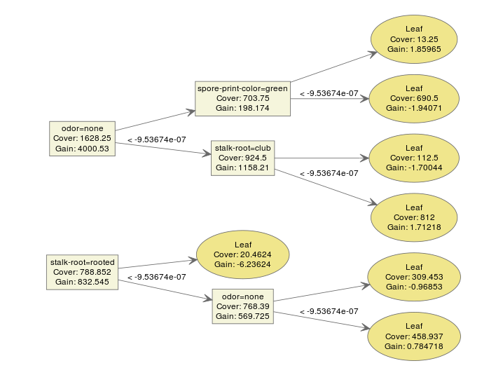
We can make an interpretation on the model easily. xgboost provides a function xgb.plot.tree to plot the model so that we can have a direct impression on the result.
However, what if we have way more trees?
bst <- xgboost(data = train$data, label = train$label, max.depth = 2,
               eta = 1, nthread = 2, nround = 10, objective = "binary:logistic")
xgb.plot.tree(feature_names = agaricus.train$data@Dimnames[[2]], model = bst)
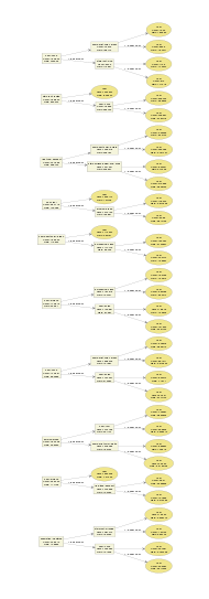
It is starting to make things messy. We even have a hard time to inspect every detail on the plot. It is not easy to tell a story with too many conditions.
Multiple-in-one plot
In xgboost, we provide a function xgb.plot.multi.trees to ensemble several trees into a single one! This function is inspired by this blogpost: https://wellecks.wordpress.com/2015/02/21/peering-into-the-black-box-visualizing-lambdamart/. This is done with the following observations:
- Almost all the trees in an ensemble model have the same shape. If the maximum depth is determined, this holds for all the binary trees.
- On each node there would be more than one feature that have appeared on this position. But we can describe it by the frequency of each feature thus make a frequenct table.
Here is an example of an “ensembled” tree visualization.
bst <- xgboost(data = train$data, label = train$label, max.depth = 15,
                 eta = 1, nthread = 2, nround = 30, objective = "binary:logistic",
                 min_child_weight = 50)
xgb.plot.multi.trees(model = bst, feature_names = agaricus.train$data@Dimnames[[2]], features.keep = 3)

The text in the nodes indicates the distribution of the features selected at this position. If we hover our mouse on the nodes, we get hte information of the path.
Feature Importance
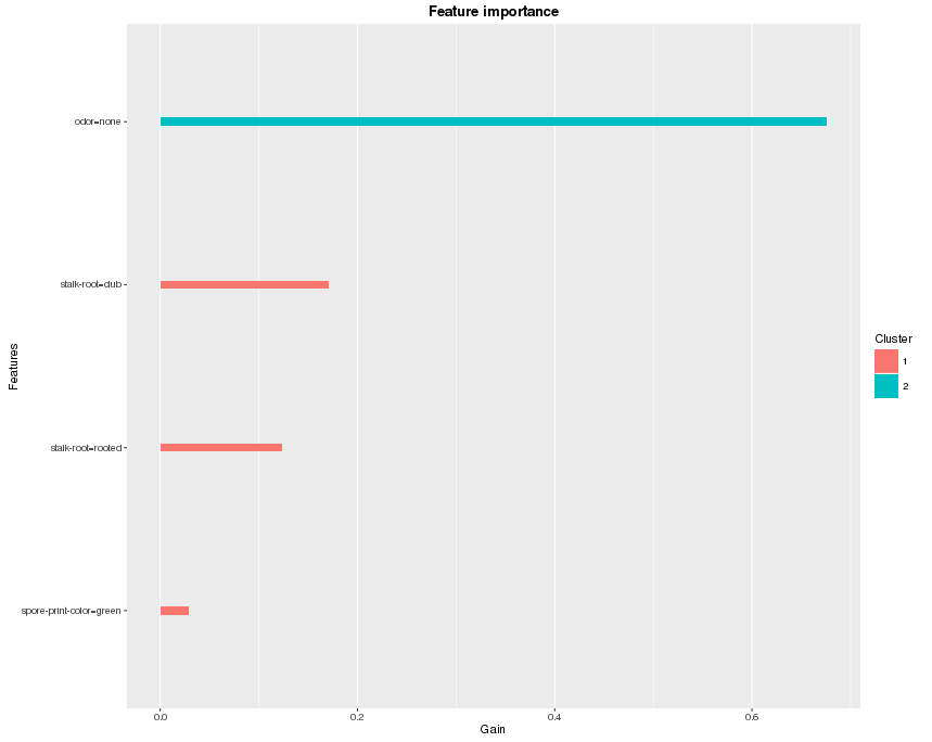
If the tree is too deep, or the number of features is large, then it is still gonna be difficult to find any useful patterns. One simplified way is to check feature importance instead. How do we define feature importance in xgboost?
In xgboost, each split tries to find the best feature and splitting point to optimize the objective. We can calculate the gain on each node, and it is the contribution from the selected feature. In the end we look into all the trees, and sum up all the contribution for each feature and treat it as the importance. If the number of features is large, we can also do a clustering on features before we make the plot. Here’s an example of the feature importance plot from the function xgb.plot.importance:
bst <- xgboost(data = train$data, label = train$label, max.depth = 2,
               eta = 1, nthread = 2, nround = 2,objective = "binary:logistic")
importance_matrix <- xgb.importance(agaricus.train$data@Dimnames[[2]], model = bst)
xgb.plot.importance(importance_matrix)
Deepness
There is more than one way to understand the structure of the trees, besides plotting them all. Since there are all binary trees, we can have a clear figure in mind if we get to know the depth of each leaf. The function xgb.plot.deepness is inspired by this blogpost: http://aysent.github.io/2015/11/08/random-forest-leaf-visualization.html.
From the function xgb.plot.deepness, we can get two plots summarizing the distribution of leaves according to the change of depth in the tree.
bst <- xgboost(data = train$data, label = train$label, max.depth = 15,
                 eta = 1, nthread = 2, nround = 30, objective = "binary:logistic",
                 min_child_weight = 50)
xgb.plot.deepness(model = bst)
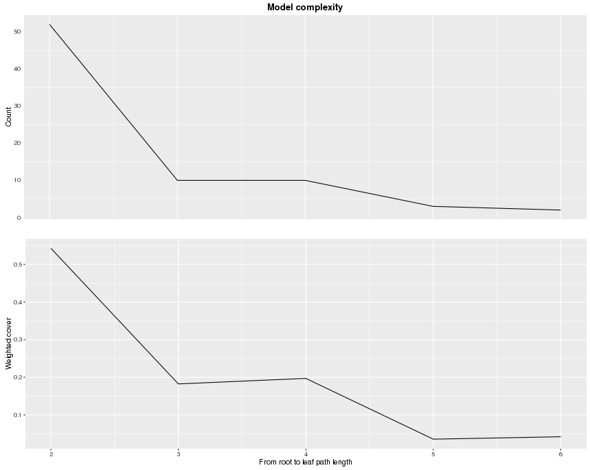
The upper plot shows the number of leaves per level of deepness. The lower plot shows noramlized weighted cover per leaf (weighted sum of instances). From this information, we can see that for the 5-th and 6-th level, there are actually not many leaves. To avoid overfitting, we can restrict the depth of trees to be a small number.
Further Readings
This blog post only brings you a glimpse on XGBoost, while there are a lot more exciting resources about it! Feel free to go through the list and look for whatever you like.
- The github repository of XGBoost
- The comprehensive documentation site for XGBoostl
- An introduction to the gradient boosting model
- Tutorials for the R package
- Introduction of the Parameters
- Awesome XGBoost, a curated list of examples, tutorials, blogs about XGBoost usecases
If there is any question, please feel free to check out the issue forum.
